Overview

Optimal control and HamPath

Let consider a simple optimal control problem with $q:=(x,v)$ the state and with $\lambda$ a parameter:

$\left\{ \begin{array}{l} \displaystyle J(u(\cdot)) = \frac{1}{2} \int_{0}^{1}u(t)^2 \mathrm{d}\, t \longrightarrow \min \\[1.0em] \displaystyle \dot{x}(t) = v(t), \\ \displaystyle \dot{v}(t) = -\lambda v(t)^2+u(t), \quad u(t) \in \mathbb{R}, \quad t \in [0,1] \text{ a.e.}, \\[1.0em] \displaystyle x(0) = -1, \quad x(1) = 0, \\ \displaystyle v(0) = \phantom{-}0, \quad v(1) = 0, \end{array} \right.$

where the initial and final times are fixed ( $t_0=0$ and $t_f=1$ ) and the boundaries are fixed to $q_0:= q(0) = (-1,0)$ and $q_f := q(1) = (0,0)$ . Define the pseudo-Hamiltonian depending on $\lambda$ :

$\begin{array}{rcl} H_\lambda:\mathbb{R}^n\times\mathbb{R}^n\times\mathbb{R} & \longrightarrow & \mathbb{R} \\ (q,p,u) & \longmapsto & \displaystyle H_\lambda(q,p,u) := p_{x} v + p_{v} (-\lambda v^2 + u) + \frac{1}{2} p^0 u^2, \end{array}$

with $n=2$ the state dimension, $p:=(p_x,p_v)$ and we fix $p^0 = -1$ (normal case). The application of the Pontryagin Maximum Principle (PMP) tells us that the minimizing trajectories $q(\cdot)$ are the projection of absolutely continuous extremals $z(\cdot) := (q(\cdot),p(\cdot))$ satisfying a.e.

$\displaystyle \dot{z}(t) = \vec{h_\lambda}(z(t))$

with

Definition 1 (Maximized Hamiltonian).

$\displaystyle h_\lambda(z) := H_\lambda(z,\bar{u}(z)) = p_{x} v + p_{v} (-\lambda v^2 + \bar{u}(z)) - \frac{1}{2}\bar{u}^2(z),$

the maximized (or true) Hamiltonian, where the optimal control is

$\displaystyle \bar{u}(z) = p_{v} = \mathrm{argmax}_{u \in \mathbb{R}} H_\lambda(z,u)$

and where the Hamiltonian system is given by

$\displaystyle \vec{h_\lambda}(z) = \left(\frac{\partial h_\lambda}{\partial p}(z), -\frac{\partial h_\lambda}{\partial q}(z)\right).$

Definition 2 (Exponential mapping). For fixed $z_0$ and $T \ge 0$ , we define in a neighborhood of $(T,z_0)$ (if possible), the following exponential mapping $(t,z_0) \mapsto \exp(t\, \vec{h_\lambda}) (z_0)$ as the trajectory $z(\cdot)$ at time $t$ satisfying the Hamiltonian system for every $s$ in $[0,t]$ , with $z(0) = z_0$ .

The minimizing curves $q(\cdot)$ are the projection of BC-extremals, i.e. extremals which satisfy the boundary conditions, and we can define the following shooting function:

Definition 3 (Shooting function).

$\begin{array}{rcl} S_{\lambda} : \mathbb{R}^n & \longrightarrow & \mathbb{R}^n \\ y & \longmapsto & \displaystyle S_{\lambda}(y) := \Pi_{q}( \exp((t_f-t_0)\, \vec{h_\lambda})(q_0,y)) - q_{f}, \end{array}$

where $\Pi_{q}$ is the canonical q-projection, i.e. $\Pi_q(z) = q$ .

The simple shooting method consists in finding a zero of the simple shooting function $S_\lambda$ , i.e. in solving $S_\lambda(y) = 0.$ This is done by Newton type methods. A zero of the simple shooting function satisfies the necessary conditions of optimality given by the PMP.

Remark 4. $S_\lambda$ depends on $\lambda$ , and we write $S(y,\lambda) := S_\lambda(y)$ the homotopic function (instead of shooting function) when we consider the parameter $\lambda$ as an independent variable. With HamPath, it is possible to solve $S(y,\lambda) = 0$ for $\lambda$ in $[0,1]$ for instance, using differential path following methods. In this case, we say that $\lambda$ is a homotopic parameter.

If we note $q(t,q_0,p_0) := \Pi_{q}( \exp(t\, \vec{h_\lambda})(q_0,p_0))$ then the trajectory $q(\cdot,q_0,p_0)$ ceases to be optimal after the time $t_c$ if $p_0$ is a critical point of the mapping $q(t_c,q_0,\cdot)$ . In this case, we name $t_c$ a conjugate time and $q(t_c,q_0,p_0)$ the associated conjugate point. Let give the following definition.

Definition 5 (Jacobi field). The differential equation on $[0,t_f]$

$\delta\dot{z}(t) = \mathrm{d} \vec{h} (z(t)) \cdot \delta z(t)$

is called a Jacobi equation, or variational system, along the extremal $z(\cdot)$ . A solution $J(\cdot)$ of the Jacobi equation along $z(\cdot)$ is called a Jacobi field and we write

$J(t) =: \exp(t\, \mathrm{d}\vec{h}|_{z(\cdot)})(J(0)).$

As a conclusion, it comes that if $t_c$ is a conjugate time then

$\displaystyle \frac{\partial q}{\partial p_0} (t_c,q_0,p_0) = \Pi_{q}\circ \exp(t_c\, \mathrm{d}\vec{h_{\lambda}} |_{z(\cdot,q_0,p_0)})(\delta z_0), \quad \delta z_0 = \begin{bmatrix} 0_n \\ I_n \end{bmatrix},$

is not of full rank $n$ .

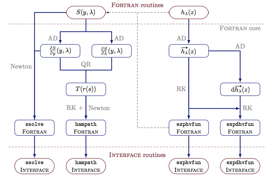
Summary of HamPath possibilities.

The idea of HamPath is to produce a collection of numerical functions in order to solve general optimal control problems. The user must only implement the maximized Hamiltonian (definition 1) and the shooting function (definition 3). The different numerical functions can be used to:

compute the solutions of the exponential mapping (definition 2);
solve the shooting equations (definition 3);
compute the set of zeros of a homotopic function (remark 4);
compute the Jacobi fields (definition 5) and check if there exists any conjugate points.

Schematic view of HamPath.

At the bottom of the following figure, the part below the doted lines is a fragment of the outputs of HamPath which is in the language chosen during the installation: it may be chosen among Fortran, Python, Matlab (only) or both Matlab and Octave. AD stands for Automatic Differentiation, RK for Runge-Kutta integrators used to solve ordinary differential equations, Newton for Newton-type methods to solve non-linear equations and QR for QR factorization.

schema